About

https://github.com/jannikmi/extremitypathfinder/actions/workflows/build.yml/badge.svg?branch=master

python package for fast geometric shortest path computation in 2D multi-polygon or grid environments based on visibility graphs.

Also see: GitHub, PyPI

License

extremitypathfinder is distributed under the terms of the MIT license (see LICENSE).

Basic Idea

Well described in [1, Ch. II 3.2]:

An environment (“world”, “map”) of a given shortest path problem can be represented by one boundary polygon with holes (themselves polygons).

IDEA: Two categories of vertices/corners can be distinguished in these kind of environments:

protruding corners (hereafter called “Extremities”)
all others

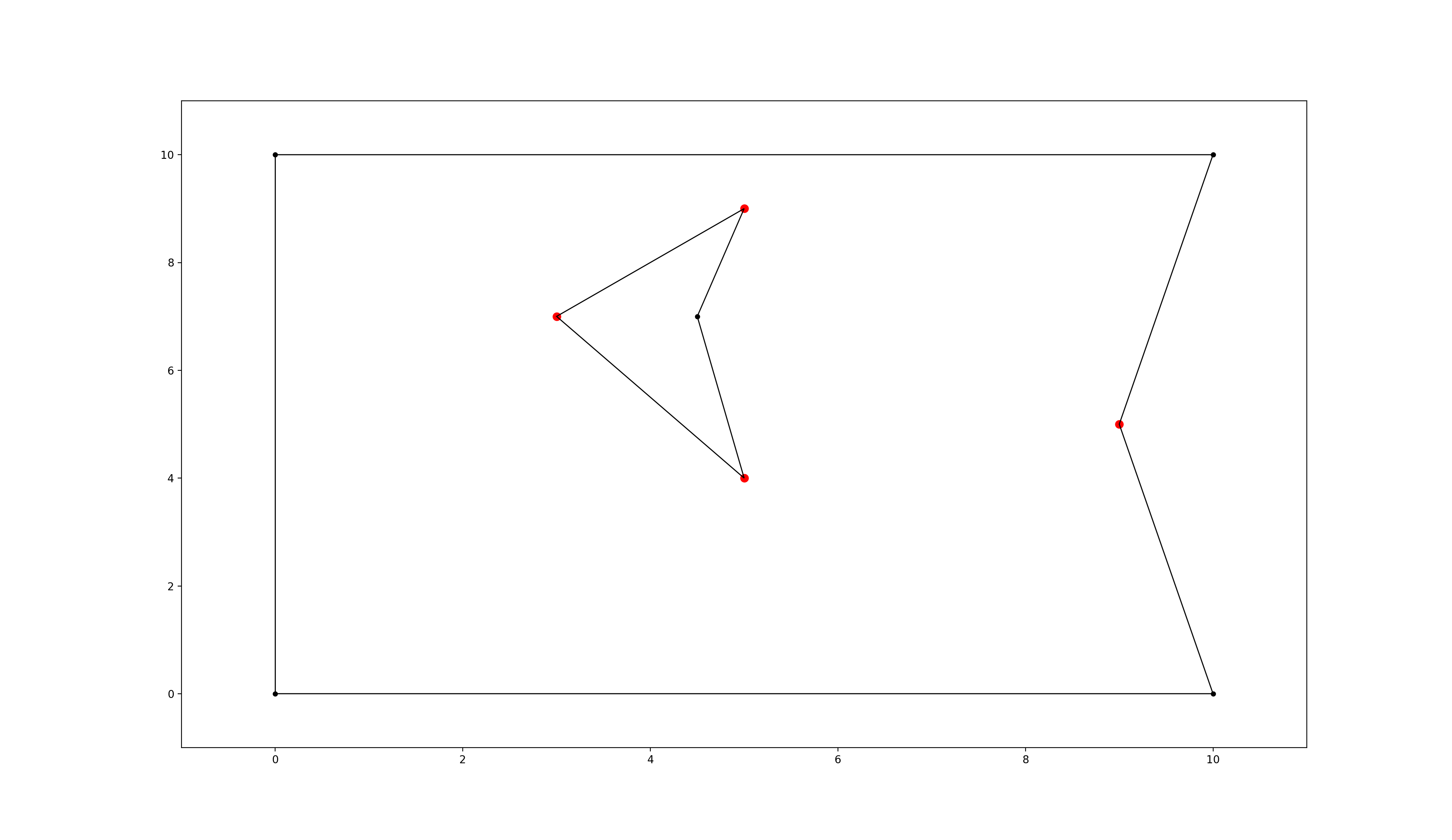
_images/map_plot.png — polygon environment with extremities marked in red

Extremities have an inner angle (facing towards the inside of the environment) of > 180 degree. As long as there are no obstacles between two points present, it is obviously always best (=shortest) to move to the goal point directly. When obstacles obstruct the direct path (goal is not directly ‘visible’ from the start) however, extremities (and only extremities!) have to be visited to reach the areas “behind” them until the goal is directly visible.

Improvement: As described in [1, Ch. II 4.4.2 “Property One”] during preprocessing time the visibility graph can be reduced further without the loss of guaranteed optimality of the algorithm: Starting from any point lying “in front of” an extremity e, such that both adjacent edges are visible, one will never visit e, because everything is reachable on a shorter path without e (except e itself). An extremity e1 lying in the area “in front of” extremity e hence is never the next vertex in a shortest path coming from e. And also in reverse: when coming from e1 everything else than e itself can be reached faster without visiting e1. -> e and e1 do not have to be connected in the graph.

Algorithm

This package pretty much implements the Visibility Graph Optimized (VGO) Algorithm described in [1, Ch. II 4.4.2], just with a few computational tweaks:

Rough Procedure:

1. Preprocessing the environment: Independently of any query start and goal points the optimized visibility graph is being computed for the static environment once. Later versions might include a faster approach to compute visibility on the fly, for use cases where the environment is changing dynamically. The edges of the precomputed graph between the extremities are shown in red in the following plots. Notice that the extremity on the right is not connected to any other extremity due to the above mentioned optimisation:

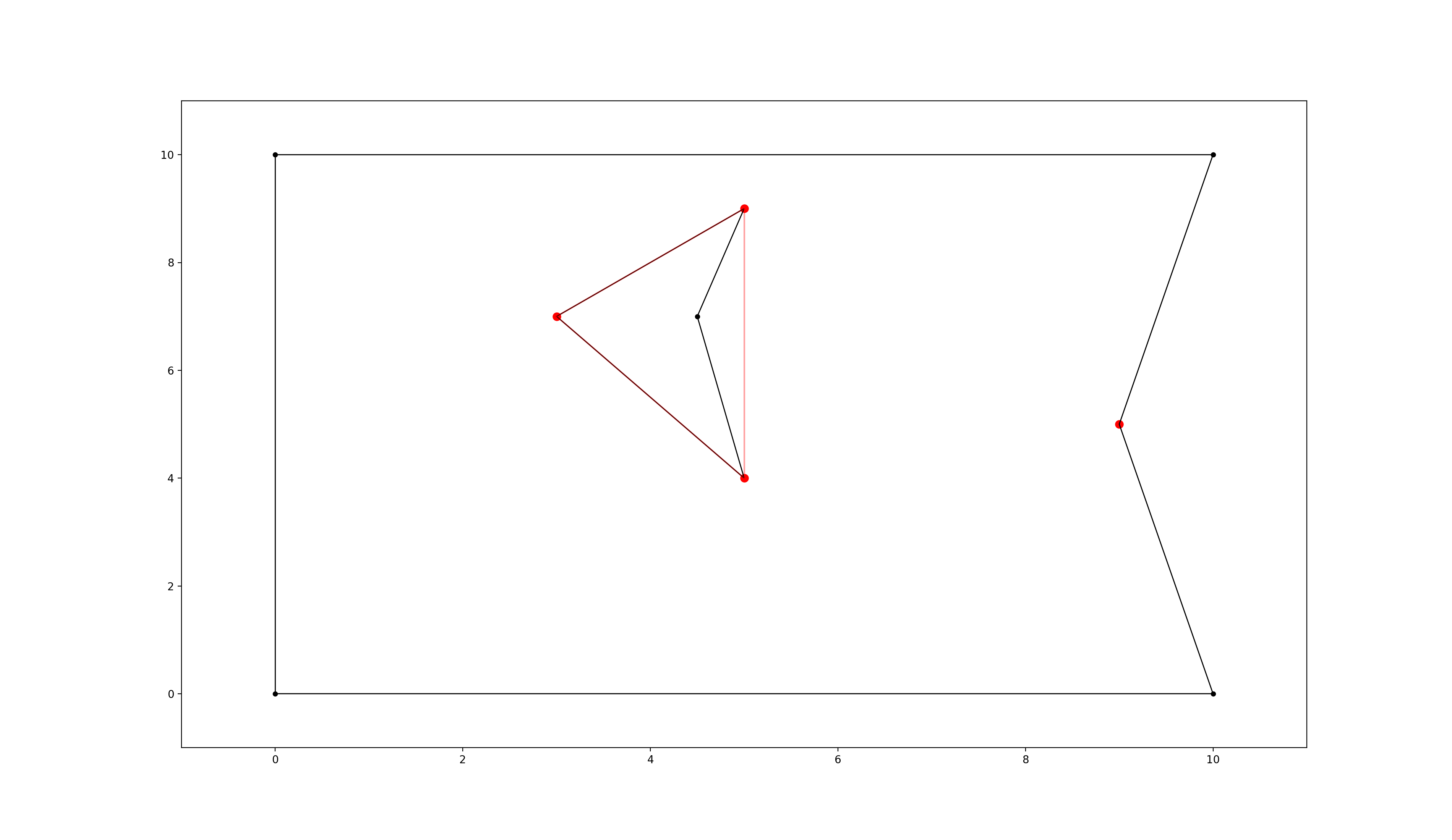
_images/prepared_map_plot.png — polygon environment with optimised visibility graph overlay in red

2. Including start and goal: For each shortest path query the start and goal points are being connected to the internal graph depending on their visibility. Notice that the added edges are directed and also here the optimisation is being used to reduce the amount of edges:

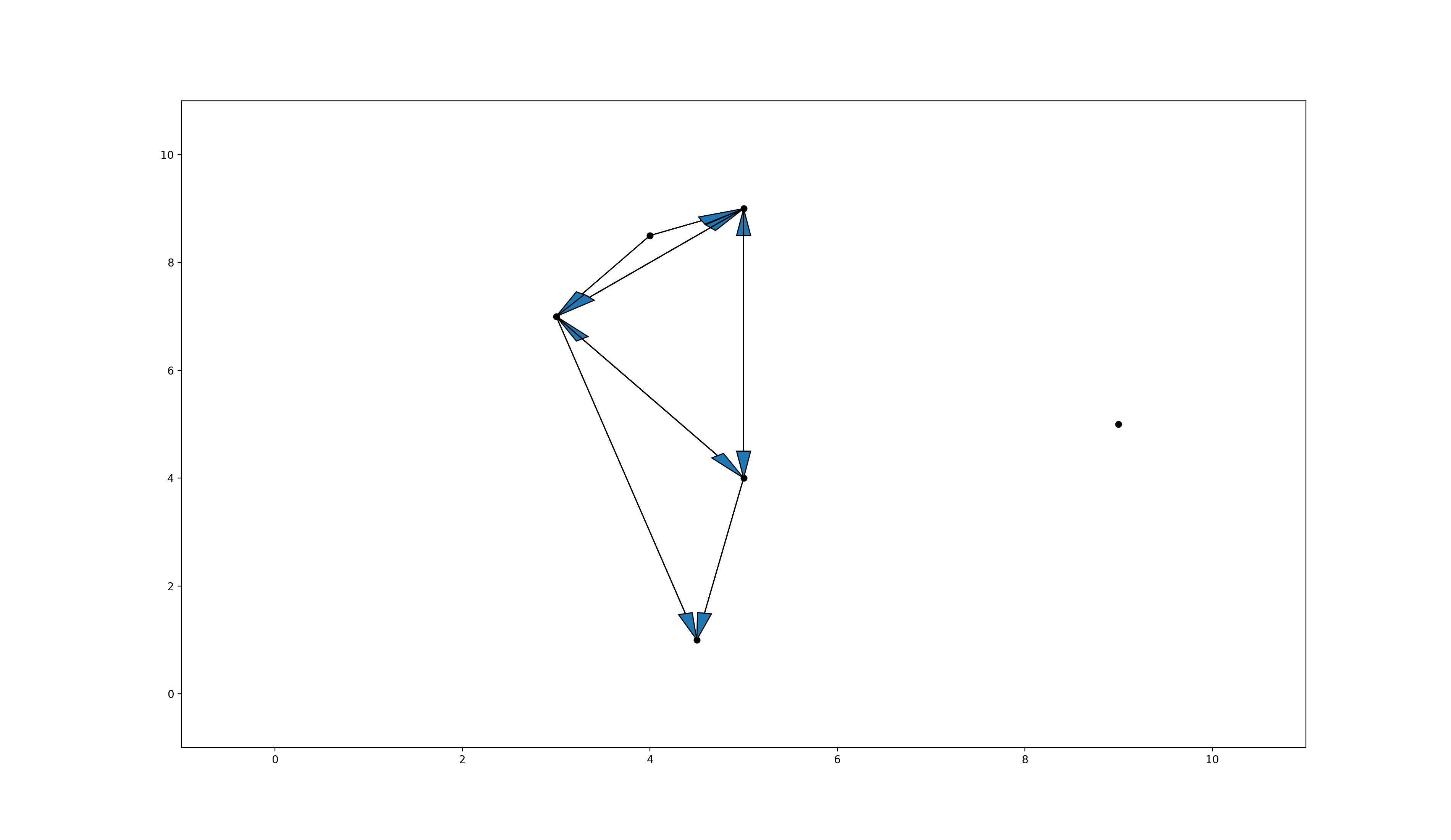
_images/graph_plot.png — optimised directed heuristic graph for shortest path computation with added start and goal nodes

3. A-star shortest path computation : Finding the shortest path on graphs is a standard computer science problem. This package uses a modified version of the popular A*-Algorithm optimized for this special use case.

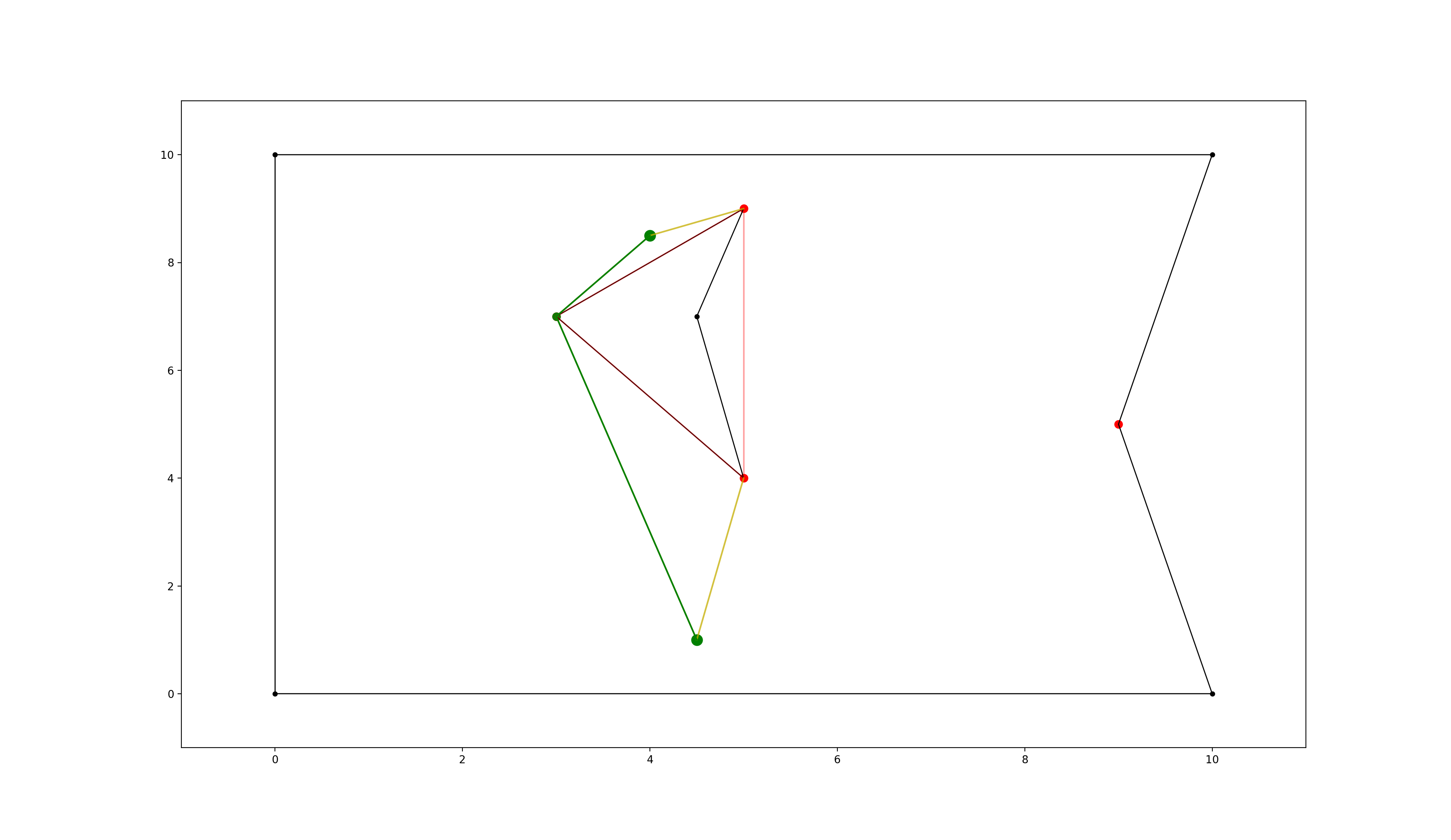
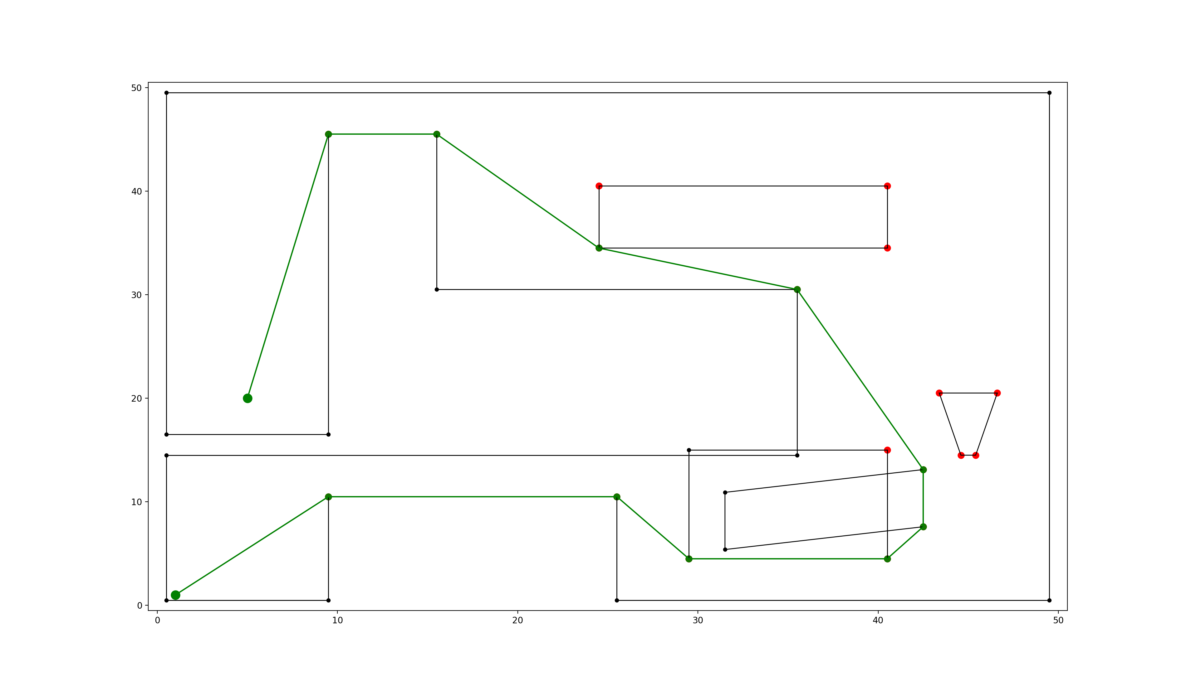
_images/graph_path_plot.png — polygon environment with optimised visibility graph overlay. visualised edges added to the visibility graph in yellow, found shortest path in green.

Edge Case: Overlapping Vertices and Edges

Warning

Overlapping edges and vertices are considered “non-blocking”. Shortest paths can run through either. Ensure Holes and Boundary Polygons are truly intersecting and not just touching in order to “block” paths.

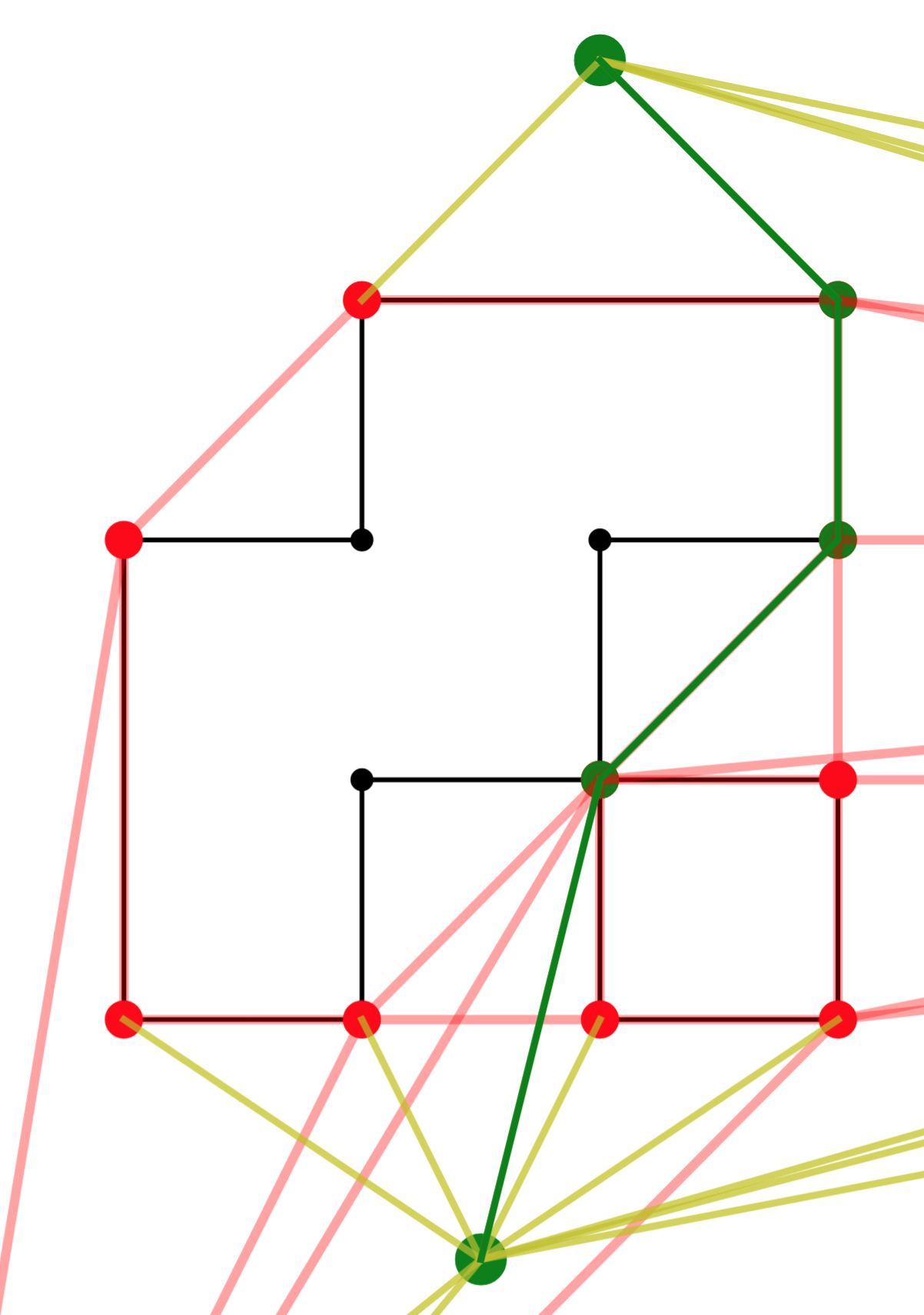
_images/path_overlapping_vertices.png — example of a shortest path running through overlapping vertices

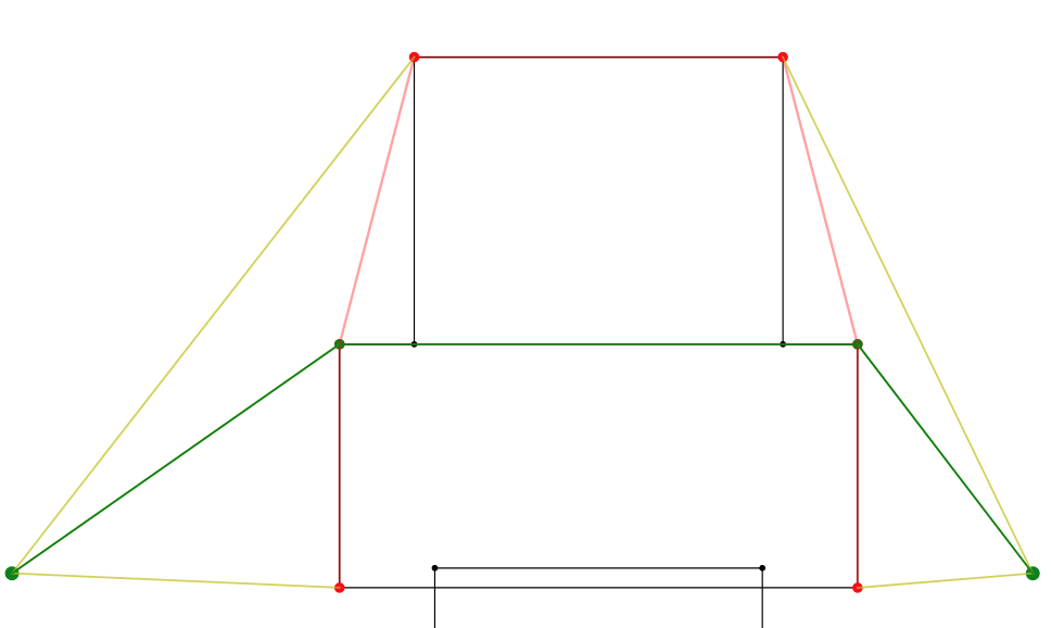
_images/path_overlapping_edges.png — example of a shortest path running along two overlapping edges

Implementation

AREA is an algorithm for computing the visibility graph.

In this use case we are not interested in the full visibility graph, but the visibility of just some points (all extremities, start and goal).

Simple fundamental idea: points (extremities) are visible when there is no edge running in front “blocking the view”.

Rough procedure: For all edges delete the points lying behind them. Points that remain at the end are visible.

Optimisations:

for each edge only checking the relevant candidates (“within the angle range”): * By sorting the edges after their angle representation (similar to Lee’s algorith, s. below), only the candidates with a bigger representation have to be checked. * By also sorting the candidates, the candidates with a smaller representation than the edge don’t have to be checked.
angle representations: instead of computing with angles in degree or radians, it is much more efficient and still sufficient to use a representation that is mapping an angle to a range \(a \in [0.0 ; 4.0[\) (\([0.0 ; 1.0[\) in all 4 quadrants). This can be done without computationally expensive trigonometric functions!
deciding if a point lies behind an edge can often be done without computing intersections by just comparing distances. This can be used to reduce the needed computations.

Properties:

checking all edges
checking an edge at most once
ability to process only a subset of all vertices as possible candidates
decreasing number of candidates after every checked origin (visibility is a symmetric relation -> only need to check once for every candidate pair!)
no expensive trigonometric computations
actual Intersection computation (solving linear scalar equations) only for a fraction of candidates
could theoretically also work with just lines (this package however currently just allows polygons)

Runtime Complexity:

\(m\): the amount of extremities (candidates)
\(n\): the amount of edges / vertices (since polynomial edges share vertices), with usually \(m << n\)
\(O(m)\) for checking every candidate as origin
\(O(n log_2 n)\) for sorting the edges, done once for every origin -> \(O(m n log_2 n)\)
\(O(n)\) for checking every edge -> \(O(m (n log_2 n + n)\)
\(O(m/n)\) (average) for checking the visibility of target candidates. only the fraction relevant for each edge will be checked -> \(O(m (n log_2 n + (n m) / n) = O(m (n log_2 n + m) = O(m n log_2 n\)
since \(m ~ n\) the final complexity is \(O(m n log_2 n) = O(n^2 log_2 n)\)

The core visibility algorithm (for one origin) is implemented in PolygonEnvironment.get_visible_idxs() in extremitypathfinder.py

Lee’s visibility graph algorithm:

complexity: \(O(n^2 log_2 n)\) (cf. these slides)

Initially all edges are being checked for intersection
Necessarily checking the visibility of all points (instead of just some)
Always checking all points in every run
One intersection computation for most points (always when T is not empty)
Sorting: all points according to degree on startup, edges in binary tree T
Can work with just lines (not restricted to polygons)

Currently using the default implementation of A* from the networkx package.

Remark: This geometrical property of the specific task (the visibility graph) could be exploited in an optimised (e.g. A*) algorithm:

It is always shortest to directly reach a node instead of visiting other nodes first
(there is never an advantage through reduced edge weight).

Make A* terminate earlier than for general graphs:

no need to revisit nodes (path only gets longer)
when the goal is directly reachable, there can be no other shorter path to it -> terminate
not all neighbours of the current node have to be checked like in vanilla A* before continuing to the next node

Comparison to pyvisgraph

This package is similar to pyvisgraph which uses Lee’s algorithm.

Pros:

very reduced visibility graph (time and memory!)
algorithms optimized for path finding
possibility to convert and use grid worlds

Cons:

parallel computing not supported so far
no existing speed comparison

Contact

Tell me if and how your are using this package. This encourages me to develop and test it further.

Most certainly there is stuff I missed, things I could have optimized even further or explained more clearly, etc. I would be really glad to get some feedback.

If you encounter any bugs, have suggestions etc. do not hesitate to open an Issue or add a Pull Requests on Git. Please refer to the contribution guidelines

References

[1] Vinther, Anders Strand-Holm, Magnus Strand-Holm Vinther, and Peyman Afshani. “Pathfinding in Two-dimensional Worlds”. no. June (2015).

Acknowledgements

Thanks to:

Georg Hess for improving the package in order to allow intersecting polygons.
Ivan Doria for adding the command line interface.